ELT: Web scraping wikipedia and ingest into SQL Server using the ELT METHOD !

In the realm of data engineering, the ELT (Extract, Load, Transform) process stands as a crucial workflow for handling and refining data. In this article, we embark on a journey through the ELT process using Python, focusing on the extraction of data from a Wikipedia source, transformation, and the subsequent loading into a SQL Server database.

Extracting Data from Wikipedia Using Python

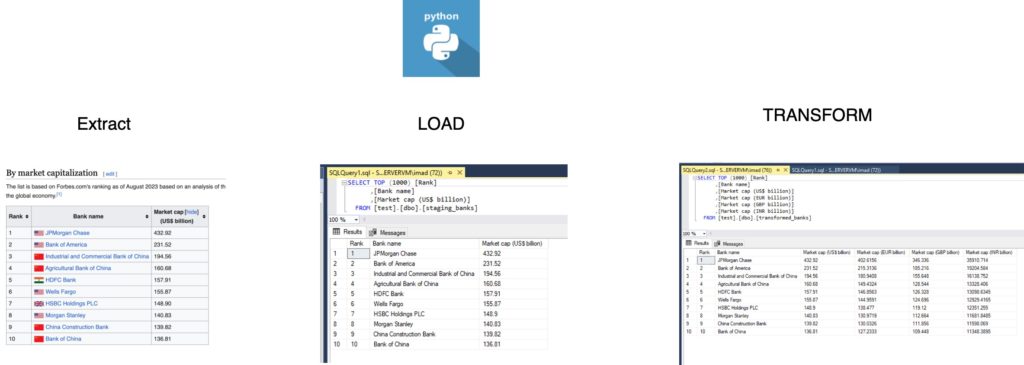
Our journey begins with extracting data from a Wikipedia page utilizing Python’s versatile libraries. The BeautifulSoup library aids in web scraping, targeting a specific table under the heading ‘By market capitalization.’

# Python Code for Data Extraction
import datetime
import pandas as pd
from bs4 import BeautifulSoup
import requests
from io import StringIO
from sqlalchemy import create_engine

# Replace these with your actual SQL Server details
SERVER = 'SQLSERVERVM\SQLEXPRESS'
DATABASE = 'test'
STAGING_TABLE_NAME = 'staging_banks'

def log_progress(message):
    timestamp = datetime.datetime.now().strftime("%Y-%m-%d %H:%M:%S")
    log_entry = f"{timestamp} : {message}\n"
    print(log_entry)  # Printing log for demonstration purposes

def extract():
    url = "https://web.archive.org/web/20230908091635/https://en.wikipedia.org/wiki/List_of_largest_banks"
    response = requests.get(url)
    soup = BeautifulSoup(response.text, 'html.parser')
    table = soup.find('span', {'id': 'By_market_capitalization'}).find_next('table')
    data = pd.read_html(StringIO(str(table)), header=0)[0]
    return data

log_progress("Starting ELT Process")

# Call the extract() function and print the returning data frame
extracted_data = extract()
log_progress("Data extracted from Wikipedia")

The code fetches the HTML content, locates the target table, and converts it into a Pandas DataFrame for further processing.

Loading Raw Data into SQL Server

Once the data is extracted, the next step involves loading it into a staging table within SQL Server. This facilitates easy access for subsequent transformation steps.

# Function to load raw data to SQL Server
def load_to_sql(engine, data, table_name):
    data.to_sql(table_name, con=engine, index=False, if_exists='replace')

# Setup database connection
connection_string = f"mssql+pyodbc://{SERVER}/{DATABASE}?driver=ODBC+Driver+17+for+SQL+Server"
engine = create_engine(connection_string)

# Call the load_to_sql() function
load_to_sql(engine, extracted_data, STAGING_TABLE_NAME)
log_progress("Raw data loaded into SQL Server")

The load_to_sql function utilizes SQLAlchemy to establish a connection and efficiently load the extracted data into a staging table.

Transforming Data for Enhanced Insights

Following the successful loading of raw data, the next phase involves transforming the data to derive valuable insights. Exchange rates are introduced, enabling the conversion of market capitalization values into various currencies.

# Function to transform data
def transform(data, exchange_rates):
    for currency, rate in exchange_rates.items():
        column_name = f"Market cap ({currency} billion)"
        data[column_name] = data['Market cap (US$ billion)'] * rate
    return data

# Read the data from SQL Server into a DataFrame
with engine.connect() as connection:
    query = f"SELECT * FROM {STAGING_TABLE_NAME}"
    raw_data_to_be_transformed = pd.read_sql_query(query, connection)

# Get exchange rates
exchange_rates_path = 'C:\\Users\\mac\\Desktop\\Data_Eng\\exchange_rate.csv'  # Replace with the actual path to your CSV
exchange_rates = get_exchange_rates(exchange_rates_path)
log_progress("Exchange rates loaded from CSV")

# Call the transform() function
transformed_data = transform(raw_data_to_be_transformed, exchange_rates)
log_progress("Data transformed with exchange rates from CSV")

Here, the transform function introduces exchange rates and computes market capitalization in various currencies.

Loading Transformed Data into SQL Server

The final step involves loading the transformed data back into SQL Server, making it readily available for analysis and reporting.

# Function to load transformed data to SQL Server
def load_transformed_to_sql(engine, data, transformed_table_name):
    data.to_sql(transformed_table_name, con=engine, index=False, if_exists='replace')

TRANSFORMED_TABLE_NAME = 'transformed_banks'
# Call the load_transformed_to_sql() function
load_transformed_to_sql(engine, transformed_data, TRANSFORMED_TABLE_NAME)
log_progress(f"Transformed data loaded into SQL Server in table {TRANSFORMED_TABLE_NAME}")

The load_transformed_to_sql function efficiently loads the transformed data into a designated table within SQL Server, creating a seamless workflow for data engineers and analysts.

Saving Transformed Data Locally

As a bonus, the transformed data is also saved to a local CSV file for convenient local access.

# Save the transformed data to CSV for local use
path_to_desktop = './transformed_data.csv'
transformed_data.to_csv(path_to_desktop, index=False)
log_progress(f"Transformed data saved to CSV at {path_to_desktop}")

This step ensures that the transformed data is accessible locally, providing flexibility for further analysis or visualization.

In conclusion, this ELT process showcases the power of Python in seamlessly handling data extraction, transformation, and loading, providing data professionals with a robust methodology for effective data management.

Full code on github : https://github.com/syedimad1998/ETL-vs-ELT